Setting Up a Simulation

Defining the Spin System

You can define a spin_system using the SpinSystem class, with which you can specify:

• The isotope, isotropic chemical shift, and scalar couplings for each spin.

• The temperature (298K by default).

• The field strength (500MHz by default).

As an example, Levitt’s Spin Dynamics describes 2,3-Dibromopropanoic acid as possessing protons with the following properties:

• 

• 

• 

• 

• 

• 

Such a spin system can be created as follows:

from nmr_sims.spin_system import SpinSystem


system = SpinSystem(
    {
        1: {
            "shift": 3.7,
            "couplings": {
                2: -10.1,
                3: 4.3,
            },
            "nucleus": "1H",
        },
        2: {
            "shift": 3.92,
            "couplings": {
                3: 11.3,
            },
            "nucleus": "1H",
        },
        3: {
            "shift": 4.5,
            "nucleus": "1H",
        },
    }
)

Setting "nucleus" = "1H" for each spin is not strictly necessary, as by default this is assumed (see the default_nucleus argument). For a description on specifying nuclei, look at nuclei.

Running a Simulation

To run a simulation, you need to import the corresponding class, which will be found in one of the submodules within experiments. For example, to perform a simple pulse-acquire experiment, you can use the PulseAcquireSimulation class, providing the spin system, along with required expriment parameters:

from nmr_sims.experiments.pa import PulseAcquireSimulation
from nmr_sims.spin_system import SpinSystem

# --snip--

sw = "2ppm"
offset = "4ppm"
points = 4096
channel = "1H"

pa_simulation = PulseAcquireSimulation(system, points, sw, offset, channel)
pa_simulation.simulate()

# The following is output to the terminal:
#
# Simulating ¹H Pulse-Acquire experiment
# --------------------------------------
# * Temperature: 298.0 K
# * Field Strength: 11.743297569643232 T
# * Sweep width: 500.000 (F1)
# * Channel 1: ¹H, offset: 2050.000 Hz
# * Points sampled: 8192 (F1)

The FID generated can then be accessed by the fid() property. A processed spectrum, along with chemical shifts and axis labels can be generated with the spectrum() method.

import matplotlib.pyplot as plt
from nmr_sims.experiments.pa import PulseAcquireSimulation
from nmr_sims.spin_system import SpinSystem


# --snip --

pa_simulation.simulate()
# Zero fill to 16k points by setting zf_factor to 2
shifts, spectrum, label = pa_simulation.spectrum(zf_factor=2)

fig, ax = plt.subplots()
ax.plot(shifts, spectrum.real, color="k")
ax.set_xlabel(label)
ax.set_xlim(reversed(ax.get_xlim()))
fig.savefig("pa_spectrum.png")

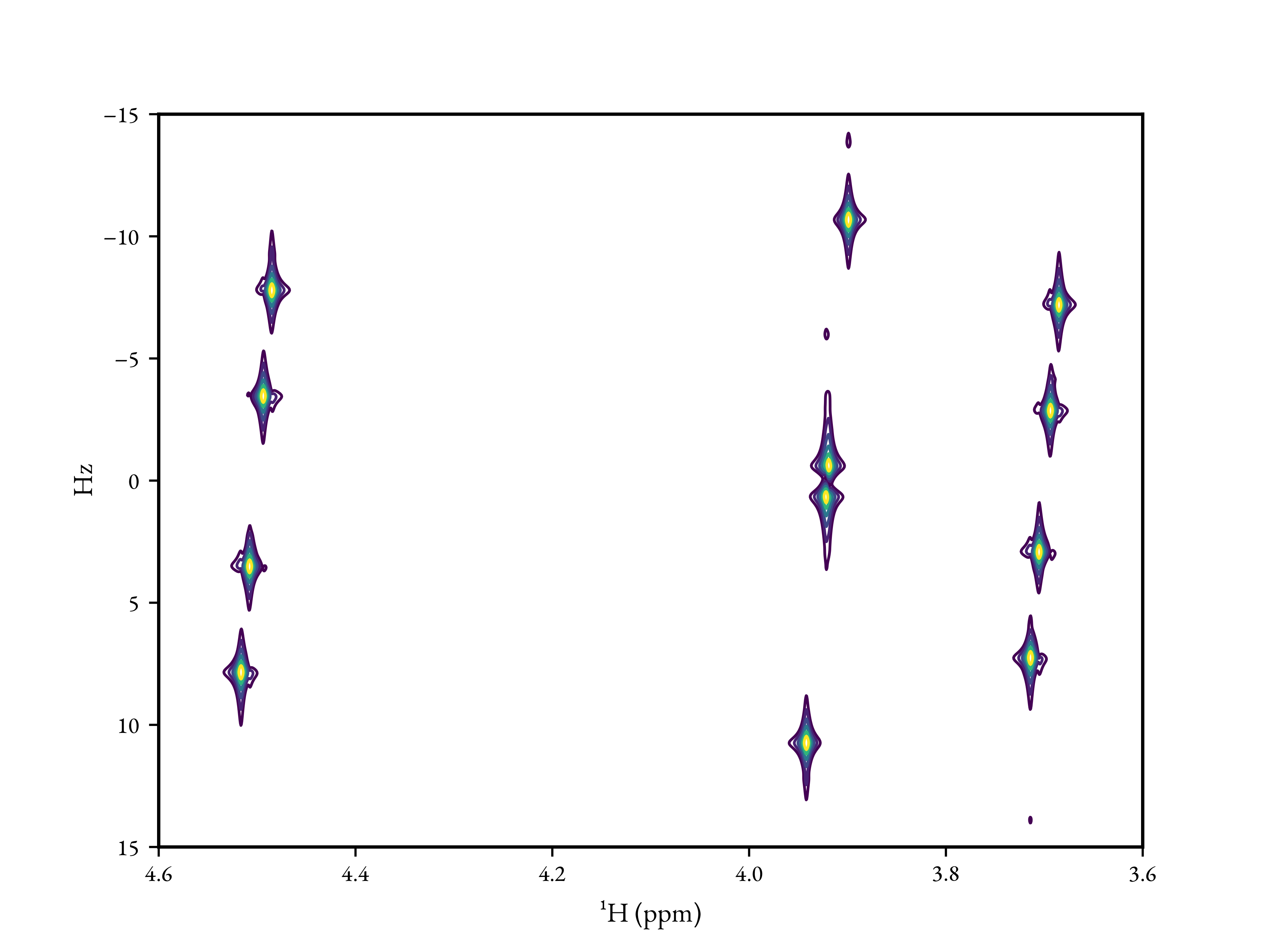
As a second example, a J-Resolved (2DJ) experiment simulation could be performed using the JresSimulation class:

import matplotlib.pyplot as plt
from nmr_sims.experiments.jres import JresSimulation
from nmr_sims.spin_system import SpinSystem


system = SpinSystem(
    {
        1: {
            "shift": 3.7,
            "couplings": {
                2: -10.1,
                3: 4.3,
            },
            "nucleus": "1H",
        },
        2: {
            "shift": 3.92,
            "couplings": {
                3: 11.3,
            },
            "nucleus": "1H",
        },
        3: {
            "shift": 4.5,
            "nucleus": "1H",
        },
    }
)

sw = ["30Hz", "1ppm"]
offset = "4.1ppm"
points = [128, 512]
channel = "1H"

# Zero pad both dimensions by a factor of 4
shifts, spectrum, labels = jres_simulation.spectrum(zf_factor=[4.0, 4.0])

# Contour level specification
nlevels = 6
base = 0.015
factor = 1.4
levels = [base * (factor ** i) for i in range(nlevels)]

# Create the figure
# N.B. spectrum() returns the data such that axis 0 (rows) correspond to F1 and
# axis 1 (columns) correspond to F2. By convention in NMR, the direct dimension
# is typically plotted on the x-axis in figures, so we need to have shifts[1] as
# x and shifts[0] as y. Also, everything has to be transposed.
fig, ax = plt.subplots()
ax.contour(shifts[1].T, shifts[0].T, spectrum.real.T, levels=levels)
ax.set_xlabel(labels[1])
ax.set_ylabel(labels[0])
ax.set_xlim(reversed(ax.get_xlim()))
ax.set_ylim(reversed(ax.get_ylim()))
fig.savefig("jres_spectrum.png")

# The following is output to the terminal:
#
# Simulating ¹H J-Resolved experiment
# -----------------------------------
# * Temperature: 298.0 K
# * Field Strength: 11.743297569643232 T
# * Sweep width: 30.000 (F1), 500.000 (F2)
# * Channel 1: ¹H, offset: 2050.000 Hz
# * Points sampled: 128 (F1), 512 (F2)