Using Estimator1D

The nmrespy.Estimator1D class is provided for the consideration of 1D NMR data.

Generating an instance

There are a few ways to create a new instance of the estimator depending on the source of the data.

Bruker data

It is possible to load both raw FID data and processed spectral data from Bruker using new_bruker(). All that is needed is the path to the dataset:

1. If you wish to import an FID, set the path as "<path_to_data>/<expno>/". There should be an fid file and an acqus file directly under this directory. The data in the fid file will be imported, and the artefact from digital filtering will be removed by a first-order phase shift.

   Note

   If you import FID data, there is a high chance that you will need to phase the data, and apply baseline correction before proceeding to run estimation. Look at phase_data() and baseline_correction(), respectively.

   >>> import nmrespy as ne
   >>> estimator = ne.Estimator1D.new_bruker("/home/simon/nmr_data/andrographolide/1")
   >>> estimator.phase_data(p0=2.653, p1=-5.686, pivot=13596)
   >>> estimator.baseline_correction()
   

2. To import processed data, set the path as "<path_to_data>/<expno>/pdata/<procno>". There should be a 1r file and a procs file directly under this directory. The data in 1r will be Inverse Fourier Transformed, and the resulting time-domain signal is sliced so that only the first half is retained.

   Note

   It can be more convienient to provide processed data, even though the data will be converted to the time-domain for estimation, as you can then rely on TopSpin’s automated processing scripts to phase and baseline correct. However, you should not apply any window function to the data other than exponential line broadening.

   >>> import nmrespy as ne
   >>> estimator = ne.Estimator1D.new_bruker("home/simon/nmr_data/andrographolide/1/pdata/1")
   >>> # Note there is no need for extra data-processing steps
   

Simulated data from a set of signal parameters

You can create an estimator with synthetic data constructed from known parameters using new_from_parameters(). The parameters must be provided as a 2D NumPy array with params.shape[1] == 4. Each row should contain a signal’s amplitude, phase (rad), frequency (Hz), and damping factor (s⁻¹).

>>> import nmrespy as ne
>>> import numpy as np
>>> # Using frequencies of 2,3-Dibromopropanoic acid @ 500MHz
>>> params = np.array([
...     [1., 0., 1864.4, 7.],
...     [1., 0., 1855.8, 7.],
...     [1., 0., 1844.2, 7.],
...     [1., 0., 1835.6, 7.],
...     [1., 0., 1981.4, 7.],
...     [1., 0., 1961.2, 7.],
...     [1., 0., 1958.8, 7.],
...     [1., 0., 1938.6, 7.],
...     [1., 0., 2265.6, 7.],
...     [1., 0., 2257.0, 7.],
...     [1., 0., 2243.0, 7.],
...     [1., 0., 2234.4, 7.],
... ])
>>> sfo = 500.
>>> estimator = ne.Estimator1D.new_from_parameters(
...     params=params,
...     pts=2048,  # FID made with 2048 points
...     sw=1.2 * sfo,  # sweep width set to 1.2 ppm
...     offset=4.1 * sfo,  # transmitter offset set to 4.1 ppm
...     sfo=sfo,  # transmitter frequecy set to 500 MHz
...     snr=40.,  # signal-to-noise ratio of the FID set to 40 dB
... )

Note

For the rest of this section, we will be using the estimator created in the above code snippet.

Simulated data from Spinach

Assuming you have installed the relevant requirements, you can create an estimator instance with data simulated using Spinach with new_spinach(). The spin system is defined by a specification of isotropic chemical shifts and scalar couplings:

• For the chemical shifts, a list of floats is required.

• For J-couplings, a list with 3-element tuples of the form (spin1, spin2, coupling) is required. N.B. the spin indices start at ``1`` rather than ``0``.

It can take some time to run this function is it involves (a) starting up MATLAB and (b) running a simulation of the experiment.

>>> import nmrespy as ne
>>> # 2,3-Dibromopropanoic acid
>>> shifts = [3.7, 3.92, 4.5]
>>> couplings = [(1, 2, -10.1), (1, 3, 4.3), (2, 3, 11.3)]
>>> sfo = 500.
>>> estimator = ne.Estimator1D.new_spinach(
...     shifts=shifts,
...     couplings=couplings,
...     pts=2048,
...     sw=1.2 * sfo,
...     offset=4.1 * sfo,
...     sfo=sfo,
... )

Viewing and accessing the dataset

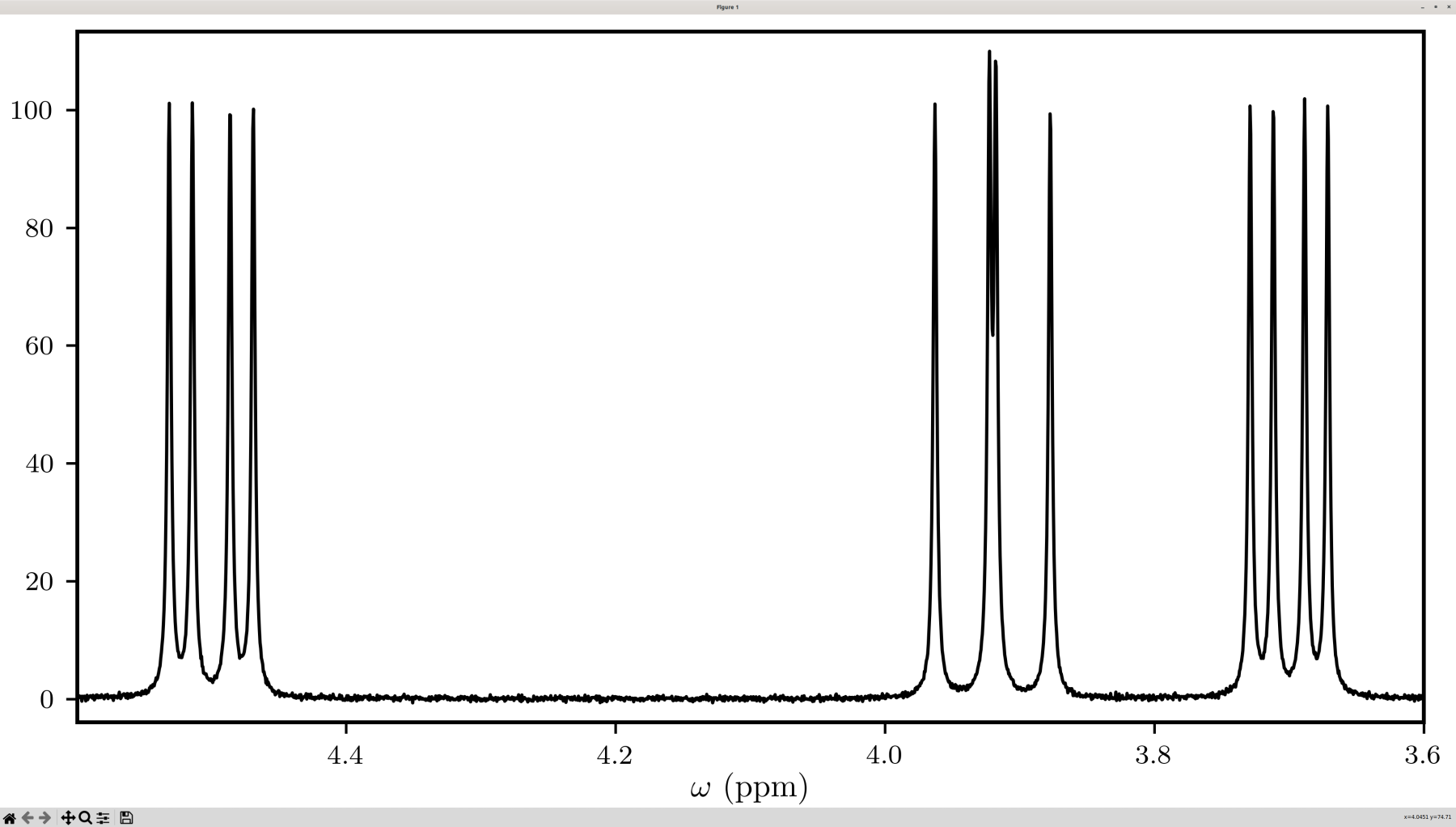
You can inspect the data associated with the estimator with view_data(), which loads an interactive matplotlib figure:

>>> estimator.view_data(freq_unit="ppm")

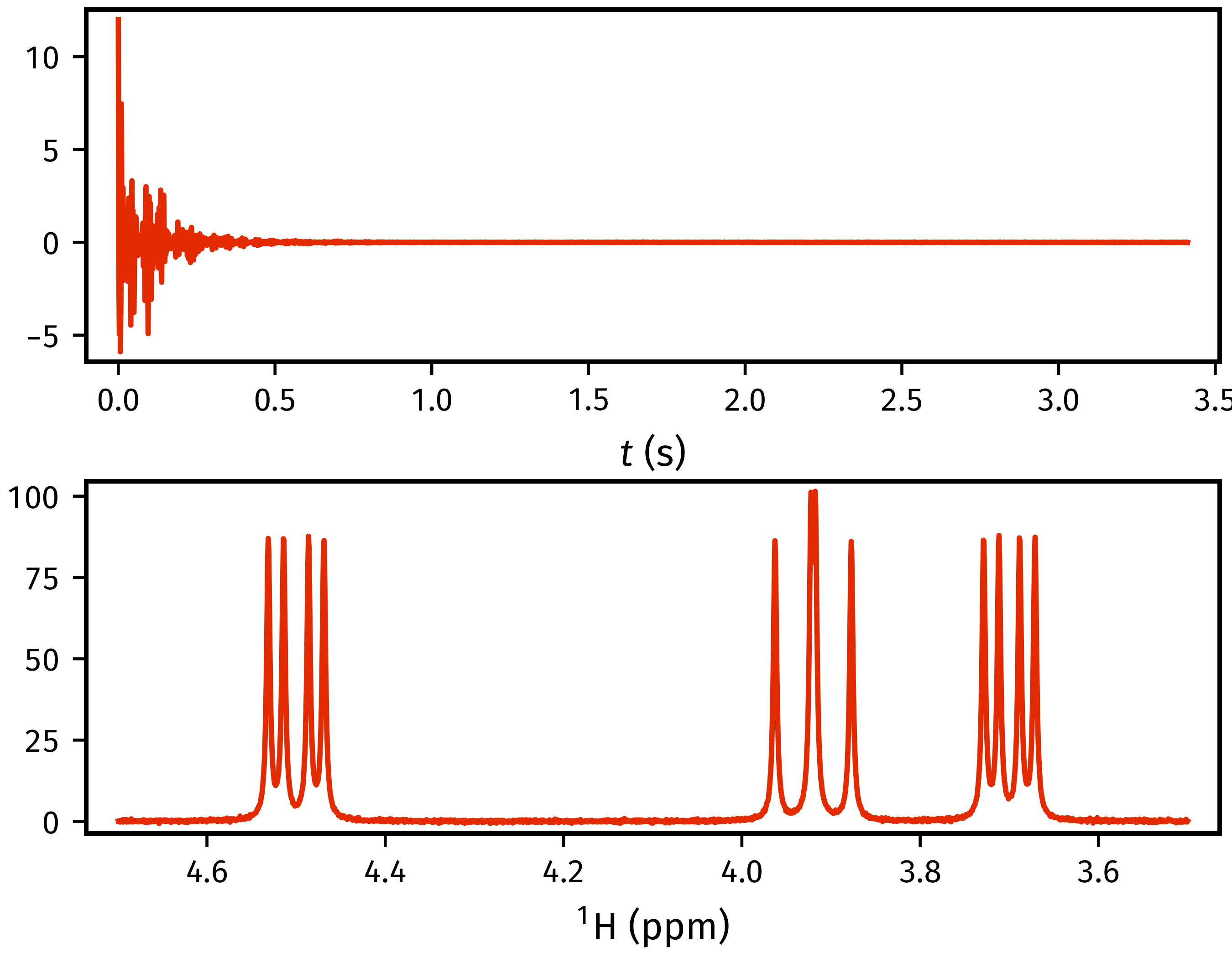
You can access the time-domain data with the data() property, and the associated time-points can be retrieved using get_timepoints(). The spectral data is accessed with spectrum(), and the corresponding chemical shifts with get_shifts().

>>> import matplotlib.pyplot as plt
>>> fid = estimator.data
>>> tp = estimator.get_timepoints()[0]
>>> spectrum = estimator.spectrum
>>> shifts = estimator.get_shifts(unit="ppm")[0]
>>> fig, axs = plt.subplots(nrows=2)
>>> axs[0].plot(tp, fid.real)
[<matplotlib.lines.Line2D object at 0x7f2c0e0aa680>]
>>> axs[0].set_xlabel("$t$ (s)")
Text(0.5, 0, '$t$ (s)')
>>> axs[1].plot(shifts, spectrum.real)
[<matplotlib.lines.Line2D object at 0x7f2c0e0aa8c0>]
>>> # Flip x-axis limits (ensure plotting from high to low shifts)
>>> axs[1].set_xlim(reversed(axs[1].get_xlim()))
(4.759384765624999, 3.4400292968749997)
>>> axs[1].set_xlabel("$^1$H (ppm)")
Text(0.5, 0, '$^1$H (ppm)')
>>> # The exact appearence of the generated figure may slightly differ to
>>> # the one below; that'll just be due to customisations I have made to mpl.
>>> plt.show()

Estimating the dataset

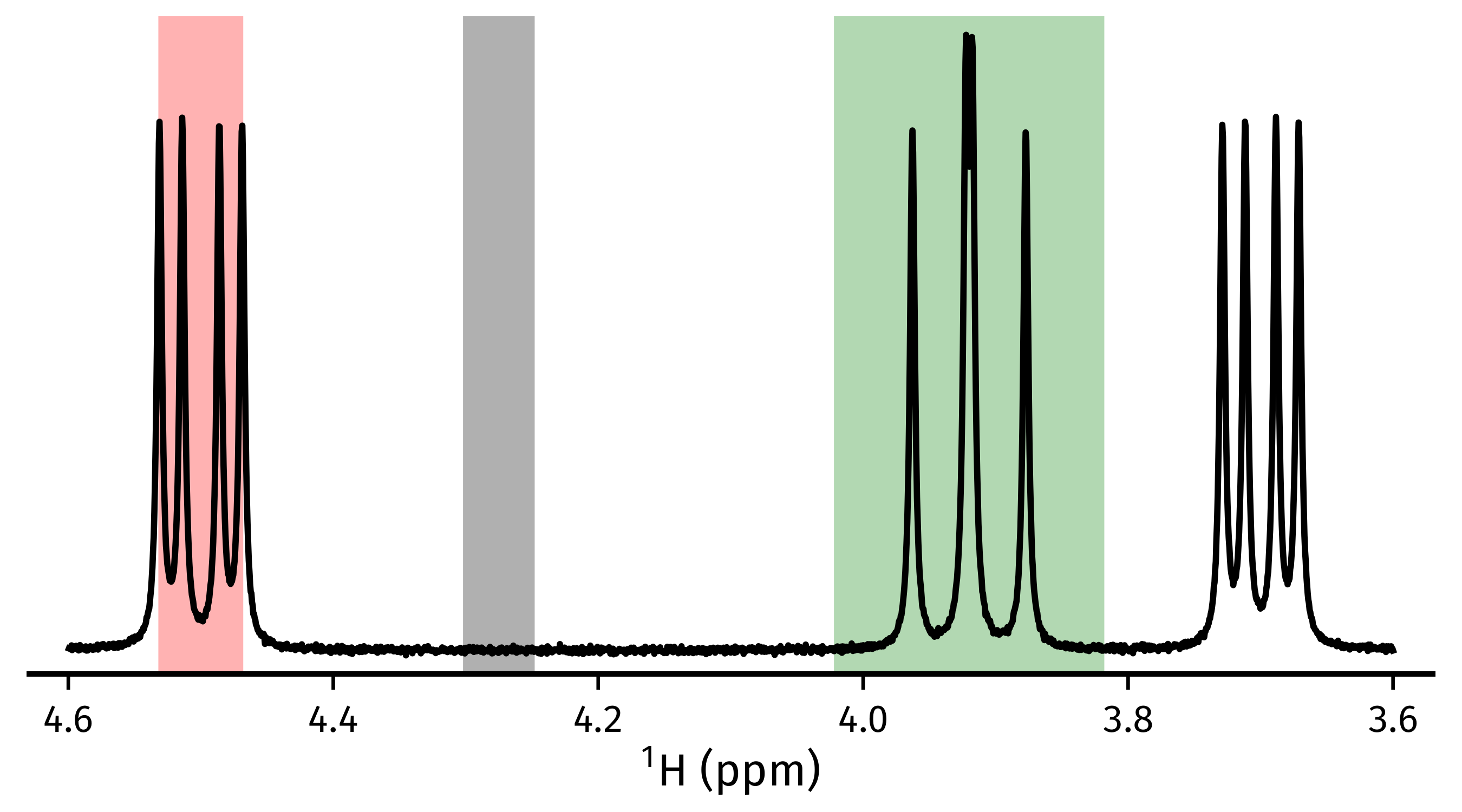
The generation of parameter estimates is facilitated using the estimate() method. In most scenarios, it will not be computationally feasible to estimate the entire FID at once, due to the number of constituent datapoints and signals. For this reason, NMR-EsPy generates frequency-filtered “sub-FIDs” to break the problem down into more manageable chunks. To create suitable sub-FIDs, it is important to select regions in which all signals of interest fully reside within its bounds. As well as this, a region that is devoid of signals (the “noise region”) must be indicated. In the figure below, the red region would be inappropriate as the signals clearly do not reside within it fully. The green region is acceptable, as the signals do abide by this. Finally, the grey region is a suitable noise region as it only comprises points in the baseline.

For our dataset, we will estimate three regions, encompassing each multiplet structure in the spectrum. Each region must be given as a tuple of 2 floats, specifying the left and right boundaries of the region of interest (the order of these doesn’t matter). By default, these are assumed to be given in Hz, unless region_unit is set to "ppm".

>>> regions = [(4.6, 4.4), (4.02, 3.82), (3.8, 3.6)]
>>> noise_region = (4.3, 4.25)
>>> for region in regions:
...     estimator.estimate(
...         region=region, noise_region=noise_region, region_unit="ppm",
...     )
...
┌─────────────────────────────────────┐
│ESTIMATING REGION: 4.6 - 4.4 ppm (F1)│
└─────────────────────────────────────┘
┌───────────┐
│MPM STARTED│
└───────────┘
--> Pencil Parameter: 125
--> Hankel data matrix constructed:
    Size:   251 x 126
    Memory: 0.4826MiB
--> Performing Singular Value Decomposition...
--> Computing number of oscillators...
    Number of oscillators will be estimated using MDL
    Number of oscillations: 4
--> Computing signal poles...
--> Computing complex amplitudes...
--> Checking for oscillators with negative damping...
    None found
┌────────────┐
│MPM COMPLETE│
└────────────┘
Time elapsed: 0 mins, 0 secs, 45 msecs
┌────────────────────┐
│OPTIMISATION STARTED│
└────────────────────┘
┌───────────────────────────┐
│TRUST NCG ALGORITHM STARTED│
└───────────────────────────┘
┌───────┬──────────────┬──────────────┬──────────────┐
│ Iter. │  Objective   │  Grad. Norm  │ Trust Radius │
├───────┼──────────────┼──────────────┼──────────────┤
│ 0     │ 0.0106245    │ 0.0653396    │ 1            │
│ 6     │ 0.00529026   │ 4.06591e-09  │ 1            │
└───────┴──────────────┴──────────────┴──────────────┘
Optimiser successfully converged.
┌────────────────────────────┐
│TRUST NCG ALGORITHM COMPLETE│
└────────────────────────────┘
Time elapsed: 0 mins, 0 secs, 34 msecs
┌─────────────────────┐
│OPTIMISATION COMPLETE│
└─────────────────────┘
Time elapsed: 0 mins, 0 secs, 101 msecs
┌───────────────────────────────────────┐
│ESTIMATING REGION: 4.02 - 3.82 ppm (F1)│
└───────────────────────────────────────┘

--snip--

┌─────────────────────────────────────┐
│ESTIMATING REGION: 3.8 - 3.6 ppm (F1)│
└─────────────────────────────────────┘

--snip--

Inspecting estimation results

Note

Result indices

Each time the estimate() method is called, the result is appended to a list containing all the generated results. For many methods that make use of estimation results, an argument called indices exists. This lets you specify the results you are interested in. By default (indices = None) all results will be used. A subset of the results can be considered by including a list of integers. For example indices = [0, 2] would mean only the 1st and 3rd results acquired with the estimator are considered.

A NumPy array of the generated results can be acquired using get_params(). The corresponding errors associated with the signal parameters are obtained with get_errors().

>>> # All params, frequencies in Hz:
>>> estimator.get_params()
[[ 1.0018e+00  1.5921e-03  1.8356e+03  7.0187e+00]
 [ 1.0003e+00  2.4881e-03  1.8442e+03  6.9968e+00]
 [ 1.0024e+00  1.5817e-03  1.8558e+03  7.0281e+00]
 [ 1.0008e+00  9.1591e-04  1.8644e+03  7.0007e+00]
 [ 1.0022e+00  7.1936e-04  1.9386e+03  7.0109e+00]
 [ 9.9470e-01 -7.4609e-04  1.9588e+03  6.9866e+00]
 [ 1.0080e+00 -1.0112e-03  1.9612e+03  7.0448e+00]
 [ 1.0009e+00 -7.1398e-04  1.9814e+03  7.0131e+00]
 [ 1.0003e+00  1.1306e-03  2.2344e+03  7.0095e+00]
 [ 1.0011e+00  6.0150e-04  2.2430e+03  7.0011e+00]
 [ 9.9902e-01  2.8231e-04  2.2570e+03  6.9856e+00]
 [ 1.0004e+00 -1.8229e-03  2.2656e+03  7.0057e+00]]
>>>
>>> # All errors, frequencies in Hz
>>> estimator.get_errors()
[[0.0013 0.0013 0.0019 0.0121]
 [0.0014 0.0014 0.002  0.0124]
 [0.0014 0.0014 0.002  0.0125]
 [0.0013 0.0013 0.0019 0.012 ]
 [0.0012 0.0012 0.0018 0.0114]
 [0.0036 0.0036 0.0034 0.0212]
 [0.0036 0.0036 0.0034 0.0213]
 [0.0012 0.0012 0.0018 0.0114]
 [0.0013 0.0013 0.0019 0.0116]
 [0.0013 0.0013 0.0019 0.0118]
 [0.0013 0.0013 0.0019 0.0118]
 [0.0013 0.0013 0.0018 0.0116]]
>>>
>>> # Params for first region, frequencies in ppm
>>> estimator.get_params(indices=[0], funit="ppm")
[[ 1.0003e+00  1.1306e-03  4.4688e+00  7.0095e+00]
 [ 1.0011e+00  6.0150e-04  4.4860e+00  7.0011e+00]
 [ 9.9902e-01  2.8231e-04  4.5140e+00  6.9856e+00]
 [ 1.0004e+00 -1.8229e-03  4.5312e+00  7.0057e+00]]
>>>
>>> # Params for second and third regions, split up
>>> estimator.get_params(indices=[1, 2], merge=False, funit="ppm")
[array([[ 1.0022e+00,  7.1936e-04,  3.8772e+00,  7.0109e+00],
       [ 9.9470e-01, -7.4609e-04,  3.9176e+00,  6.9866e+00],
       [ 1.0080e+00, -1.0112e-03,  3.9224e+00,  7.0448e+00],
       [ 1.0009e+00, -7.1398e-04,  3.9628e+00,  7.0131e+00]]),
 array([[1.0018e+00, 1.5921e-03, 3.6712e+00, 7.0187e+00],
       [1.0003e+00, 2.4881e-03, 3.6884e+00, 6.9968e+00],
       [1.0024e+00, 1.5817e-03, 3.7116e+00, 7.0281e+00],
       [1.0008e+00, 9.1591e-04, 3.7288e+00, 7.0007e+00]])]

Writing result tables

Tables of parameters can be saved to .txt and .pdf formats. using write_result(). For PDF generation, you will need a working LaTeX installation. See the installation instructions.

>>> for fmt in ("txt", "pdf"):
...     estimator.write_result(
...         path="tutorial_1d",
...         fmt=fmt,
...         description="Simulated 2,3-Dibromopropanoic acid signal.",
...     )
...
Saved file tutorial_1d.txt.
Saved file tutorial_1d.tex.
Saved file tutorial_1d.pdf.
You can view and customise the corresponding TeX file at tutorial_1d.tex.

• tutorial_1d.txt: Text file.

• tutorial_1d.pdf: PDF file.

• tutorial_1d.tex: TeX file used to generate the PDF

Creating result plots

Figures giving an overview of the estimation result can be generated using plot_result().

>>> for (txt, indices) in zip(("complete", "index_1"), (None, [1])):
...     fig, ax = estimator.plot_result(
...         indices=indices,
...         figure_size=(4.5, 3.),
...         region_unit="ppm",
...         axes_left=0.03,
...         axes_right=0.97,
...         axes_top=0.98,
...         axes_bottom=0.09,
...     )
...     fig.savefig(f"tutorial_1d_{txt}_fig.pdf")
...

• tutorial_1d_complete_fig.pdf: result for all regions considered

• tutorial_1d_index_1_fig.pdf: result for 2nd estimated region only (index 1)

Saving the estimator

The estimator object itself can be saved and reloaded for future use with the to_pickle() and from_pickle() methods, respectively:

>>> estimator.to_pickle("tutorial_1d")
Saved file tutorial_1d.pkl.
>>> # Load the estimator and assign to the `estimator_cp` variable
>>> estimator_cp = ne.Estimator1D.from_pickle("tutorial_1d")

• tutorial_1d.pkl

Saving a logfile

A logfile listing all the methods called on the estimator can be created using save_log():

>>> estimator.save_log("tutorial_1d")
Saved file tutorial_1d.log.

• tutorial_1d.log

The full script

Everything covered here is incorporated into the following Python script: estimator1d_tutorial.py